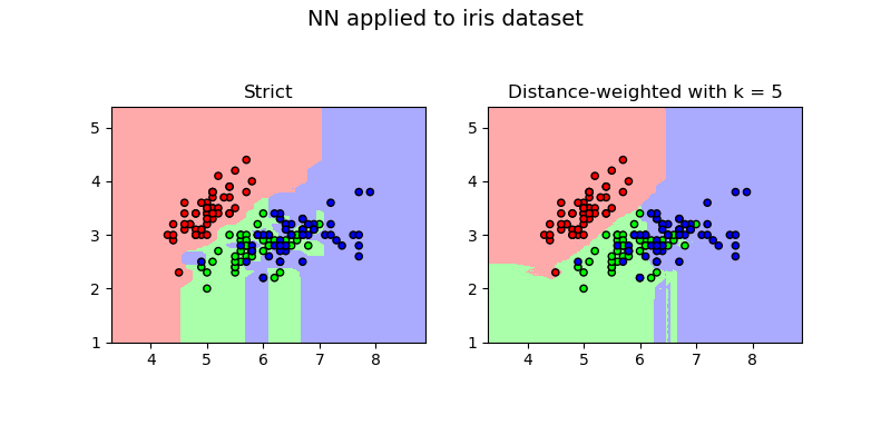
Multiclass classification with NN

The figures contain the training instances within a section of the selected feature space. The training instances are coloured according to their true labels, while the feature space is coloured according to predictions on the basis of the training instances, making the decision boundaries visible.

Two subfigures are displayed: the first represents strict NN (k == 1), while the second represents distance-weighted NN with k == 5.

print(__doc__)

import numpy as np
import matplotlib.pyplot as plt
from matplotlib.colors import ListedColormap
from sklearn import datasets

from frlearn.base import select_class
from frlearn.classifiers import NN

# Import example data and reduce to 2 dimensions.
iris = datasets.load_iris()
X = iris.data[:, :2]
y = iris.target

# Define color maps.
cmap_light = ListedColormap(['#FFAAAA', '#AAFFAA', '#AAAAFF'])
cmap_bold = ListedColormap(['#FF0000', '#00FF00', '#0000FF'])

# Initialise figure with wide aspect for two side-by-side subfigures.
plt.figure(figsize=(8, 4))

for i, distance_weighted, k, title in [
    (1, False, 1, 'Strict'),
    (2, True, 20, 'Distance-weighted with k = 5')
]:
    axes = plt.subplot(1, 2, i)

    # Create an instance of the NN classifier and construct the model.
    clf = NN(distance_weighted=distance_weighted, k=k, )
    model = clf(X, y)

    # Create a mesh of points in the attribute space.
    step_size = .02
    x_min, x_max = X[:, 0].min() - 1, X[:, 0].max() + 1
    y_min, y_max = X[:, 1].min() - 1, X[:, 1].max() + 1
    xx, yy = np.meshgrid(np.arange(x_min, x_max, step_size), np.arange(y_min, y_max, step_size))

    # Query mesh points to obtain class values and select highest valued class.
    Z = model(np.c_[xx.ravel(), yy.ravel()])
    Z = select_class(Z, labels=model.classes)

    # Plot mesh.
    Z = Z.reshape(xx.shape)
    plt.pcolormesh(xx, yy, Z, cmap=cmap_light)

    # Plot training instances.
    plt.scatter(X[:, 0], X[:, 1], c=y, cmap=cmap_bold,
                edgecolor='k', s=20)

    # Set subplot aspect to standard aspect ratio.
    axes.set_aspect(1.0 / axes.get_data_ratio() * .75)

    # Set plot dimensions.
    plt.xlim(xx.min(), xx.max())
    plt.ylim(yy.min(), yy.max())

    # Describe the subfigures.
    plt.title(title)

plt.suptitle('NN applied to iris dataset', fontsize=14)
plt.show()